BYU CS classes

To understand MCMC and Hamiltonian MCMC.

You need to install the autograd package. This can be installed with pip install autograd.

For this lab, you will implement two variants of MCMC inference: basic Metropolis Hastings and Hamiltonian MCMC. Your notebook should present visualizations of both the resulting samples, as well as plots of the state over time.

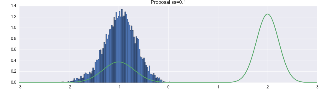
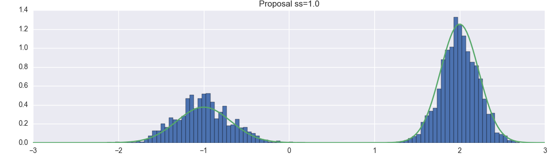
For example, here are my visualization of basic Metropolis-Hastings, with different proposal parameters:

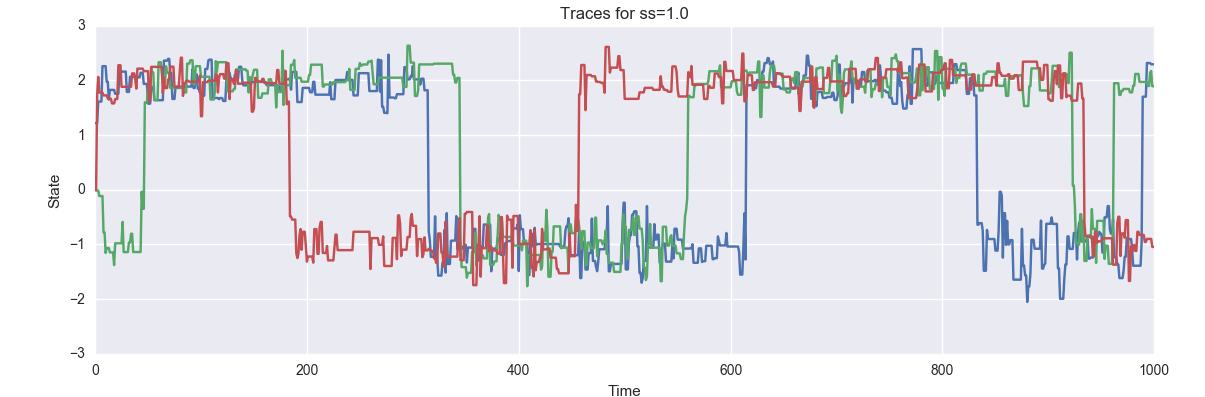
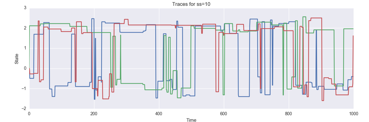
And here are plots of the resulting state evolution over time:

Your notebook should produce similar plots for the HMC algorithm, although you only need to produce two plots (one histogram, and one state evolution plot, instead of three of each). So to clarify, your notebook should have 6 plots for part one (three histograms, three evolution plots) and two plots for part two (one histogram, one evolution plot).

Your notebook should also include a small writeup of your results, as described below.

Your notebook will be graded on the following elements:

• 25% Correct implementation of Metropolis Hastings inference
• 5% Correct calculation of gradients
• 45% Correct implementation of Hamiltonian MCMC
• 15% A small write-up comparing and contrasting MH, HMC, and the different proposal distributions
• 10% Final plot is tidy and legible

For this lab, you will code two different MCMC algorithms. Each will attempt to draw samples from the same distribution, given by the following density function:

import numpy as np
def p( x, temperature=1.0 ):
    return np.exp( -10*temperature*((x-2)**2) ) + 0.3*np.exp( -0.5*10*temperature*((x+1)**2) )

This distribution has two modes that are separated by a region of low probability.

Part 1: Metropolis Hastings

For this part, you should implement the basic MH MCMC algorithm. You should use a Gaussian proposal distribution with three different variances (0.1, 1.0 and 10.0). Your sampler should start with an initial state of 0.

For each different proposal distribution, you should run your MCMC chain for 10,000 steps, and record the sequence of states. Then, you should produce a visualization of the distribution of states, and overlay a plot of the actual target distribution. They may or may not match (see, for example, the first example plot in the Description section).

Furthermore, for each proposal distribution, you should run three independent chains (you can do these sequentially or in parallel, as you like). You should display each of these three chains on a single plot with time on the x-axis and the state on the y-axis. Ideally, you will see each of the three chains mixing between two modes; you may notice other features of the behavior of the samplers as well, which you should report in your writeup!

Part 2: Hamiltonian MCMC

For this part, you will code the Hamiltonian MCMC algorithm, as discussed in class. You will run three independent chains and report them in the same graphs. To do this, you will need to compute the gradient of the density function with respect to the state. An easy easy way to do this is to use the autograd package:

from autograd import grad
import autograd.numpy as np
grad_p = grad( p )

The function grad_p accepts the same parameters as p, but it returns the gradient, instead of the density.

You should use the leapfrog method to integrate the dynamics.

Remember that you will need to introduce as many momentum variables as there are state (ie, position) variables.

A detailed explanation of Hamiltonian MCMC can be found here:Hamiltonian MCMC.

• You will find the equations describing the leapfrog method in Equations 5.18, 5.19 and 5.20.
• You will find a description of how to convert a given p(x) into a Hamiltonian in Section 5.3.1.
• You will find a description of the complete HMC algorithm in section 5.3.2.1

Remember that you will alternate between two steps:

1. Sampling the momentum conditioned on the position. This is just sampling from a Gaussian.
2. Proposing a new state for the position, given the momentum. This involves integrating the dynamics, and then accepting or rejecting based on integration error.

You will have to tune two parameters in order to implement HMC: the variance of the momentum variables, and the timestep used for integrating the dynamics. Experiment with both, and report your results using plots like those you prepared for Part 1.

Part 3: Observations

You have now coded two different inference algorithms, and a few variants of each. For this section, you must provide a small write-up that compares and contrasts each. Answer at least the following questions:

1. What was the acceptance rate of each algorithm? (ie, what percentage of proposals were accepted)
2. Why don't some inference algorithms explore both modes of the density?
3. Why do some algorithms stay in the same state repeatedly? Is this good or bad?
4. What were the best values for the variance of the momentum variables and the timestep you found? How did you know that they were good?

You may find plt.hist with the normed=True option helpful.