BYU CS classes

To understand how to use kernel density estimation to both generate a simple classifier and a class-conditional visualization of different hand-written digits.

You should turn in an iPython notebook that performs three tasks. All tasks will be done using the MNIST handwritten digit data set (see Description for details):

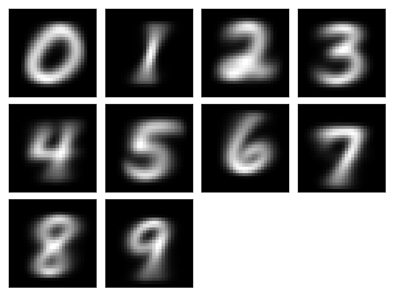
1. Generate a visualization of the expected value of each class, where the density over classes is estimated using a kernel density estimator (KDE). The data for these KDEs should come from the MNIST training data (see below). Your notebook should generate 10 images, arranged neatly, one per digit class. Your image might look something like the one on the right.
2. Build a simple classifier using only the class means, and test it using the MNIST test data. (Note: this couldn't possibly be a good classifier!) That is, for each test data point $x_j$, you should compute the probability that $x_j$ came from a Gaussian centered at $\mu_k$, where $\mu_k$ is the expected value of class $k$ you computed in Part (1). Classify $x_j$ as coming from the most likely class. Question: does the variance of your kernel matter?
3. Build a more complex classifier using a full kernel density estimator. For each test data point $x_j$, you should calculate the probability that it belongs to class $k$. Question: does the variance of your kernel matter?

Note: Part (3) will probably run slowly! Why? To make everyone's life easier, only run your full KDE classifier on the first 1000 test points.

For Part (2) and Part (3) your notebook should report two things:

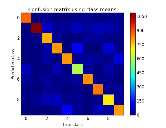
1. The overall classification rate. For example, when I coded up Part 2, my classification error rate was 17.97%. When I coded up Part (3), my error rate was 3.80% 4.0%. (if you omit the factor of 1/2 in the exponent, you get 3.8%)
2. A confusion matrix (see MLAPP pg. 183), or this wikipedia article. A confusion matrix is a complete report of all of the different ways your classifier was wrong, and is much more informative than a single error rate; for example, a confusion matrix will report the number of times your classifier reported “3”, when the true class was “8”. You can report this confusion matrix either as a text table, or as an image. My confusion matrix is shown to the right; you can see that my classifier generally gets things right (the strong diagonal), but sometimes predicts “9” when the true class is “4” (for example).

What errors do you think are most likely for this lab?

Somewhere in the first 1000 training images is an outlier! Using the tools of kernel density estimation and anomaly detection, can you find it? (To get credit for this, you cannot manually look for the outlier, you must automatically detect it; your notebook should contain the code you used to do this.)

If so, have your notebook display an image with the outlier, along with the index of the outlier.

Note: if you find the outlier, please don't tell other students which one it is!

Your notebook will be graded on the following:

• 10% Correct calculation of class means
• 5% Tidy and legible visualization of class means
• 20% Correct implementation of simple classifier
• 40% Correct implementation of full KDE classifier
• 15% Correct calculation of confusion matrix
• 10% Tidy and legible confusion matrix plots

• 10% Extra credit for outlier detection

For this lab, you will be experimenting with Kernel Density Estimators (see MLAPP 14.7.2). These are a simple, nonparametric alternative to Gaussian mixture models, but which form an important part of the machine learning toolkit.

At several points during this lab, you will need to construct density estimates that are “class-conditional”. For example, in order to classify a test point $x_j$, you need to compute

$$p( \mathrm{class}=k | x_j, \mathrm{data} ) \propto p( x_j | \mathrm{class}=k, \mathrm{data} ) p(\mathrm{class}=k | \mathrm{data} ) $$

where

$$p( x_j | \mathrm{class}=k, \mathrm{data} )$$

is given by a kernel density estimator derived from all data of class $k$.

The data that you will analyzing is the famous MNIST handwritten digits dataset. You can download some pre-processed MATLAB data files from the class Dropbox, or via direct links below:

MNIST training data vectors and labels

MNIST test data vectors and labels

These can be loaded using the scipy.io.loadmat function, as follows:

import scipy.io
 
train_mat = scipy.io.loadmat('mnist_train.mat')
train_data = train_mat['images']
train_labels = train_mat['labels']
 
test_mat = scipy.io.loadmat('mnist_test.mat')
test_data = test_mat['t10k_images']
test_labels = test_mat['t10k_labels']

The training data vectors are now in train_data, a numpy array of size 784×60000, with corresponding labels in train_labels, a numpy array of size 60000×1.

Here is a simple way to visualize a digit. Suppose our digit is in variable X, which has dimensions 784×1:

import matplotlib.pyplot as plt
plt.imshow( X.reshape(28,28).T, interpolation='nearest', cmap="gray")

Here are some functions that may be helpful to you:

import matplotlib.pyplot as plt
plt.subplot
 
numpy.argmax
 
numpy.exp
 
numpy.mean
 
numpy.bincount