This is an old revision of the document!
Table of Contents
Objective:
To understand state space models, and in particular, the Kalman filter.
Pre-requisite:
You must install the python skimage package. This can be installed via conda install skimage.
Deliverable:
For this lab, you will implement the Kalman filter algorithm on two datasets. Your notebook should produce two visualizations of the observations, the true state, the estimated state, and your estimate of the variance of your state estimates.
For the first dataset, you will implement a simple random accelerations model and use it to track a simple target. Your final visualization should look something like the following:

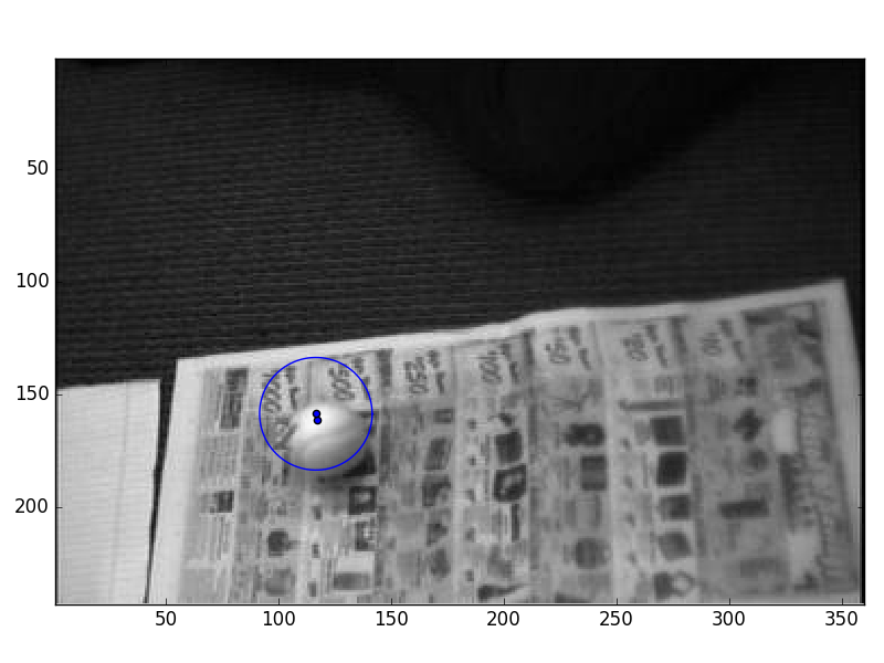
For the second dataset, you will use a series of '(x,y)' observations that were derived from a vision processing task. For this dataset, you will need to set the parameters of your filter to whatever best values you can, and then show a visualization of the result. The visualization of the result should consist of two parts:
- First, a series of frame snapshots showing the estimated position and uncertainty
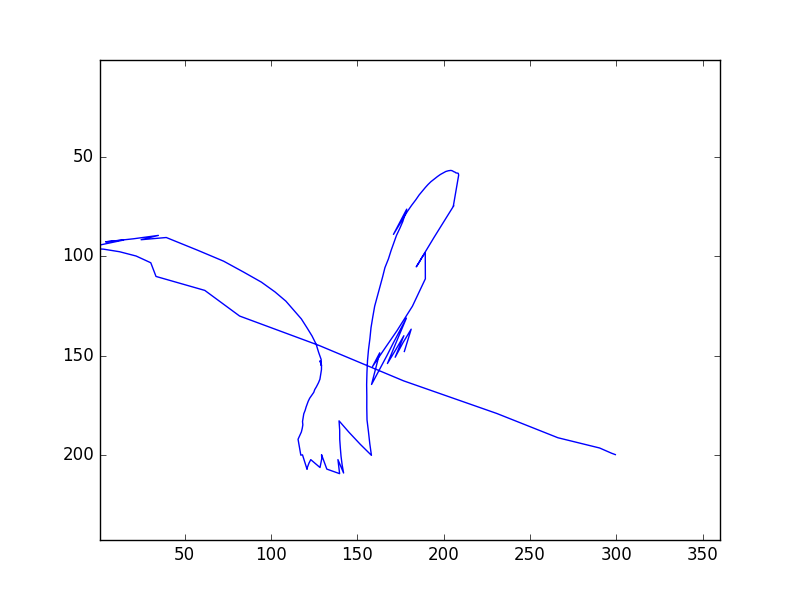
- Second, a plot of how the ball moved around in the field of view
Examples of both are here:
Grading:
Your notebook will be graded on the following elements:
- 20% Kalman gain is correctly computed
- 20% State is correctly updated
- 20% Covariance is correctly computed
- 20% State and covariance are correctly recorded
- 20% Final plot is tidy and legible
Description - first dataset:
For the first dataset, you will perform simple target tracking using the random accelerations model. You should use the equations given in Lecture 17. The data can be found here:
There are two arrays in this .mat file: data contains the actual (noisy) observations at each timestep, while true_data contains the true x,y coordinates at each timestep. Note that your kalman filter should only use the noisy observations; the true x,y coordinates are only given for visualization purposes.
To visualize the uncertainty at each timestep, the code for plotting the 95% confidence interval of a Gaussian, from lab 6, can be used.
The model is given by
# our dynamics are described by random accelerations
A = np.asarray([
    [ 1, 0, 1, 0, 0.5, 0 ],
    [ 0, 1, 0, 1, 0, 0.5 ],
    [ 0, 0, 1, 0, 1, 0 ],
    [ 0, 0, 0, 1, 0, 1 ],
    [ 0, 0, 0, 0, 1, 0 ],
    [ 0, 0, 0, 0, 0, 1 ] ])

# our observations are only the position components
C = np.asarray([
    [1, 0, 0, 0, 0, 0],
    [0, 1, 0, 0, 0, 0]])

# our dynamics noise tries to force random accelerations to account
# for most of the dynamics uncertainty
Q = 1e-2 * np.eye( 6 )
Q[4,4] = 0.5  # variance of accelerations is higher
Q[5,5] = 0.5

# our observation noise
R = 20 * np.eye( 2 )

# initial state
mu_t = np.zeros(( 6, 1 ))
sigma_t = np.eye( 6 )
Description - second dataset:
With your Kalman filtering code in hand, the second dataset is relatively straightforward. This is a chance for you to experiment with the parameters of the model and see how good of a tracker you can build.
The dataset is derived from a sequence of images, which can be downloaded here:
The data is a sequence of images of a ball rolling across a camera's field of view. We'd like to implement a tracker for the ball, but there's no way we can cope with images in the framework of the Kalman filter. Instead, we'll do a brief pre-processing step: we'll use template matching to search for the ball in each frame of video, and record the best (x,y) position of the template match.
Unfortunately, template matching is noisy and imprecise - so we'll need to filter the resulting location estimates.
Here is the code to load the data and perform template matching:
import numpy as np
import scipy.io
import skimage.feature
import matplotlib
import matplotlib.pyplot as plt

tmp = scipy.io.loadmat('ball_data.mat')
frames = tmp['frames']  # frames of our video
ball = tmp['ball']  # our little template

data = []
for i in range( 0, frames.shape[1] ):
    tmp = np.reshape( frames[:,i], (360,243) ).T  # slurp out a frame
    ncc = skimage.feature.match_template( tmp, ball )  # create a normalized cross correlation image
    maxloc = np.unravel_index( tmp.argmax(), tmp.shape )  # find the point of highest correlation
    data.append( maxloc )  # record the results

data = np.asarray( data )
Now, you can run your Kalman filter on the (x,y) coordinates in the data matrix.
Hints:
To avoid numerical instabilities in the calculation of your covariance matrices, you may want to use np.linalg.pinv.
Here's a little snippet of code that will make a movie, showing the ball rolling and the Gaussian position estimate superimposed:
# assumes that "mus" contains a list of Gaussian means, and that "covs" is a list of Gaussian covariances

for t in range(0, data.shape[0]):

    tmp = np.reshape( frames[:,t], (360,243) ).T

    plt.figure(1)
    plt.clf()
    plt.imshow( tmp, interpolation='nearest', cmap=matplotlib.cm.gray )
    plt.scatter( data[t][1], data[t][0] )
    plt.scatter( mus[t][1], mus[t][0] )

    foo = cov_to_pts( covs[t][0:2,0:2] )

    plt.plot( foo[0,:] + mus[t][1], foo[1,:] + mus[t][0] )
    plt.xlim([1, 360])
    plt.ylim([243,1])

    plt.pause(0.01)
