This is an old revision of the document!
Table of Contents
Objective:
To understand particle filters, and to gain experience with debugging likelihoods.
Suggested pre-requisite:
You may wish to install the python pyqtgraph package. This can be installed via conda install pyqtgraph. This is a plotting package that is significantly faster than matplotlib when scatter plotting many points (ie, particles).
Deliverable:
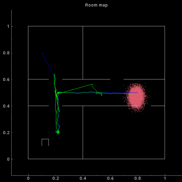
For this lab, you will implement a particle filter for robot localization. Your notebook should print a visualization of the true location of the robot, your estimate of its position, and a simple scatterplot of the distribution of particles at the end of tracking. For example, my visualization looks like the following:
To successfully complete the lab, you will have to:
- Create an initial set of particles
- Create a proposal distribution
- Create an observation likelihood distribution
- Given a set of particles, compute the expected value of the x,y position of the robot
- Resample the particles to avoid weight degenercy
Grading standards:
Your notebook will be graded on the following elements:
- 25% Implemented a correct sensor likelihood
- 25% Implemented a reasonable proposal distribution
- 30% Implemented particle resampling correctly
- 10% Correctly compute expected value of state x,y coordinates
- 10% Final plot is tidy and legible
Description:
For this lab, you will need the following files:
sensors.mat contains the data you will use (you can also regenerate it directly, using the script below). The data is in the sonars field, and the true states are in the true_states field. true_states is a 3xT matrix, where each 3×1 column represents the true x,y and angle (\in 0,2*pi) of the robot at time t.
lab8_common.py contains utility functions that will enable you to create a simple map, and compute what a robot would see from a given position and angle.
lab8_gen_sonars.py is the script that I used to generate the data for this lab. If you run it, it will generate a new dataset, but it will also produce a nice visualization of the robot as it moves around, along with what the sensors measure.
To get started, check out the provided functions in lab8_common.py. There are two critical functions:
create_mapwill create a map object and return itcast_rayswill simulate what a robot would see from a specific x,y,theta position, given a map
cast_rays is fully vectorized, meaning that you can simulate from multiple locations simultaneously. For example, in my code, I only call cast_rays once:
    part_sensor_data = cast_rays( parts, room_map )
    liks = ray_lik( data[:,t:t+1], part_sensor_data.T ).T
where I have represented my particles as a 3xN matrix. In the above example call, part_sensor_data is an Nx11 matrix. ray_lik is my implementation of the likelihood function $p(y_t|z_t)$, and is also fully vectorized. It returns an Nx1 matrix, with the likelihood of each particle.
Your proposal distribution can be anything you want. Be creative. You may have to experiment!
You should experiment with two different likelihoods. First, try using a simple Gaussian likelihood. Second, try using a simple Laplacian distribution. (The Laplacian is like a Gaussian, except that instead of squaring the difference, one uses an absolute value).
You will have to experiment with the parameters of these distributions to make them work. Try values between 0.01 and 1.
Hints:
You may find the numpy.random.mtrand.multinomial function helpful.
It can be frustrating to experiment with a particle filter when the interface is too slow. By using pyqtgraph instead of matplotlib, you can speed things up considerably.
Here is some code to create a pyqtgraph window, and show the map.
from pyqtgraph.Qt import QtGui, QtCore
import pyqtgraph as pg

app = QtGui.QApplication( [] )
win = pg.GraphicsWindow( title="Particle filter" )
win.resize( 600, 600 )
win.setWindowTitle( 'Particle filter' )
pg.setConfigOptions( antialias=True )

p3 = win.addPlot( title="Room map" )

for i in range( 0, room_map.shape[0] ):
    p3.plot( [room_map[i,0], room_map[i,2]], [room_map[i,1], room_map[i,3]] )
p3.setXRange( -0.1, 1.1 )
p3.setYRange( -0.1, 1.1 )
To speed things up further, you should use the .setData method on your plots. This replaces the data used for a particular plotting element, and is faster than deleting and recreating the plot element. This is particularly important when trying to update many particles.
Here's a snippet of my code. ts_plot and ex_plot are initialized to None. My particles are stored in a 3xN matrix called parts, my expected states are stored in a 3xt matrix called exs.
if ts_plot == None:
    ts_plot = p3.plot( true_states[0,0:t+1], true_states[1,0:t+1], pen=(0,0,255) )
    ex_plot = p3.plot( exs[0,0:t+1], exs[1,0:t+1], pen=(0,255,0) )
    pts = p3.scatterPlot( parts[0,:], parts[1,:], symbol='o', size=1, pen=(255,100,100) )

else:
    ts_plot.setData( true_states[0,0:t+1], true_states[1,0:t+1] )
    ex_plot.setData( exs[0,0:t+1], exs[1,0:t+1] )
    pts.setData( parts[0,:], parts[1,:] )

pg.QtGui.QApplication.processEvents()
(you must call processEvents to actually update the display)
The combination of these two things allowed me to experiment with my particle filter in real-time. Note that you are not required to produce any sort of visualization over time, just a single plot at the end of running your code. The use of pyqtgraph is strictly for the work you will do debugging your particle filter.
