BYU CS classes

To understand the LDA model and Gibbs sampling.

For this lab, you will implement Gibbs sampling on the LDA model. You will use as data a set of about 400 General Conference talks.

Your notebook should implement two different inference algorithms on the LDA model: (1) a standard Gibbs sampler, and (2) a collapsed Gibbs sampler.

Your notebook should produce a visualization of the topics it discovers, as well as how those topics are distributed across documents. You should highlight anything interesting you may find! For example, when I ran LDA with 10 topics, I found the following topic

GS Topic 3:
                it    0.005515
          manifest    0.005188
             first    0.005022
            please    0.004463
        presidency    0.004170
          proposed    0.003997
                 m    0.003619
             favor    0.003428
           sustain    0.003165
           opposed    0.003133

To see how documents were assigned to topics, I visualized the per-document topic mixtures as a single matrix, where color indicates probability:

Here, you can see how documents that are strongly correlated with Topic #3 appear every six months; these are the sustainings of church officers and statistical reports.

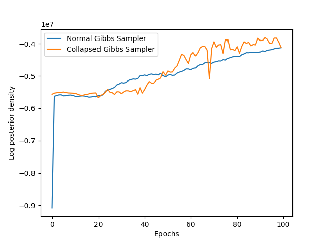
Your notebook must also produce a plot of the log posterior of the data over time, as your sampler progresses. You should produce a single plot comparing the regular Gibbs sampler and the collapsed Gibbs sampler.

To the right is an example of my log pdfs.

Your notebook will be graded on the following elements:

• 40% Correct implementation of Gibbs sampler
• 40% Correct implementation of collapsed Gibbs sampler
• 20% Final plots are tidy and legible (at least 2 plots: posterior over time for both samplers, and heat-map of distribution of topics over documents)

For this lab, you will code two different inference algorithms on the Latent Dirichlet Allocation (LDA) model.

You will use a dataset of general conference talks. Download and untar these files; there is helper code in the Hints section to help you process them.

Part 1: Basic Gibbs Sampler

The LDA model consists of several variables: the per-word topic assignments, the per-document topic mixtures, and the overall topic distributions. Your Gibbs sampler should alternate between sampling each variable, conditioned on all of the others. Equations for this were given in the lecture slides.

Hint: it may be helpful to define a datastructure, perhaps called civk, that contains counts of how many words are assigned to which topics in which documents. My civk datastructure was simply a 3 dimensional array.

You should run 100 sweeps through all the variables.

Note: this can be quite slow. As a result, you are welcome to run your code off-line, and simply include the final images / visualizations in your notebook (along with your code, of course!).

Part 2: Collapsed Gibbs Sampler

The collapsed Gibbs sampler integrates out the specific topic and per-document-topic-distribution variables. The only variables left, therefore, are the per-word topic assignments. A collapsed Gibbs sampler therefore must iterate over every word in every document, and resample a topic assignment.

Again, computing and maintaining a datastructure that tracks counts will be very helpful. This will again be somewhat slow.

Here is some starter code to help you load and process the documents, as well as some scaffolding to help you see how your sampler might flow.

import numpy as np
import re
 
vocab = set()
docs = []
 
D = 472 # number of documents
K = 10 # number of topics
 
# open each file; convert everything to lowercase and strip non-letter symbols; split into words
for fileind in range( 1, D+1 ):
    foo = open( 'output%04d.txt' % fileind ).read()    
    tmp = re.sub( '[^a-z ]+', ' ', foo.lower() ).split()
    docs.append( tmp )
 
    for w in tmp:
        vocab.add( w )
 
# vocab now has unique words
# give each word in the vocab a unique id
ind = 0
vhash = {}
vindhash = {}
for i in list(vocab):
    vhash[i] = ind
    vindhash[ind] = i
    ind += 1
 
# size of our vocabulary
V = ind
 
# reprocess each document and re-represent it as a list of word ids
 
docs_i = []
for d in docs:
    dinds = []
    for w in d:
        dinds.append( vhash[w] )
    docs_i.append( dinds )
 
# ======================================================================
 
qs = randomly_assign_topics( docs_i, K )
 
alphas = np.ones((K,1))[:,0]
gammas = np.ones((V,1))[:,0]
 
# topic distributions
bs = np.zeros((V,K)) + (1/V)
# how should this be initialized?
 
# per-document-topic distributions
pis = np.zeros((K,D)) + (1/K)
# how should this be initialized?
 
for iters in range(0,100):
    p = compute_data_likelihood( docs_i, qs, bs, pis)
    print("Iter %d, p=%.2f" % (iters,p))
 
    # resample per-word topic assignments bs
 
    # resample per-document topic mixtures pis
 
    # resample topics