This is an old revision of the document!
Table of Contents
Objective:
To read current papers on DNN research and translate them into working models. To experiment with DNN-style regularization methods, including Dropout, Dropconnect, and L1 weight regularization.
Deliverable:
For this lab, you will need to implement three different regularization methods from the literature, and explore the parameters of each.
- You must implement dropout (NOT using the pre-defined Tensorflow layers)
- You must implement dropconnect
- You must implement L1 weight regularization
You should turn in an iPython notebook that shows three plots, one for each of the regularization methods.
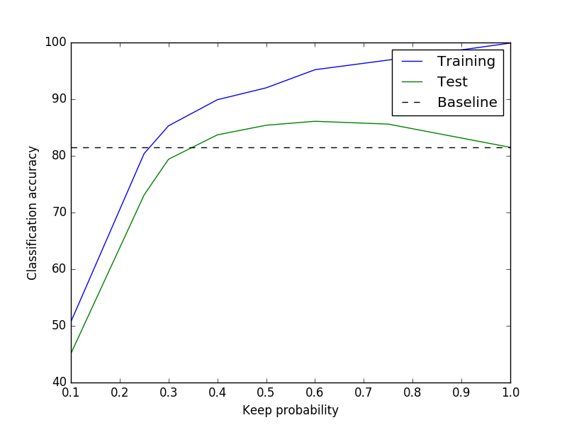
- For dropout: a plot showing training / test performance as a function of the “keep probability”.
- For dropconnect: the same
- For L1 a plot showing training / test performance as a function of the regularization strength, \lambda
An example of my training/test performance for dropout is shown at the right.
NOTE: because this lab can be more computationally time consuming than the others (since we're scanning across parameters), you are welcome to turn in your plots and your code separately. (This means, for example, that you can develop and run all of your code using an IDE other than the Jupyter notebook, collect the data, and then run a separate little script to generate the plots. Or, a particularly enterprising student may use his or her new supercomputer account to sweep all of the parameter values in parallel (!) ). You will need to zip up your images and code into a single file for submission to Learning Suite.
Grading standards:
Your notebook will be graded on the following:
- 40% Correct implementation of Dropout
- 30% Correct implementation of Dropconnect
- 20% Correct implementation of L1 regularization
- 10% Tidy and legible plots
Description:
This lab is a chance for you to start reading the literature on deep neural networks, and understand how to replicate methods from the literature. You will implement 4 different regularization methods, and will benchmark each one.
To help ensure that everyone is starting off on the same footing, you should download the following scaffold code:
For all 4 methods, we will run on a single, deterministic batch of the first 1000 images from the MNIST dataset. This will help us to overfit, and will hopefully be small enough not to tax your computers too much.
Part 1: implement dropout
For the first part of the lab, you should implement dropout. The paper upon which you should base your implementation is found at:
The relevant equations are found in section 4 (pg 1933). You may also refer to the slides.
There are several notes to help you with this part:
- First, you should run the provided code as-is. It will overfit on the first 1000 images (how do you know this?). Record the test and training accuracy; this will be the “baseline” line in your plot.
- Second, you should add dropout to each of the
h1,h2, andh3layers. - You must consider carefully how to use tensorflow to implement dropout.
- Remember that when you test images (or when you compute training set accuracy), you must scale activations by the
keep_probability, as discussed in class and in the paper. - You should use the Adam optimizer, and optimize for 150 steps.
Note that although we are training on only the first 1000 images, we are testing on the entire 10,000 image test set.
In order to generate the final plot, you will need to scan across multiple values of the keep_probability. You may wish to refactor the provided code in order to make this easier. You should test at least the values [ 0.1, 0.25, 0.5, 0.75, 1.0 ].
Once you understand dropout, implementing it is not hard; you should only have to add ~10 lines of code.
Also note that because dropout involves some randomness, your curve may not match mine exactly; this is expected.
Part 2: implement dropconnect
The specifications for this part are similar to part 1. Once you have implemented Dropout, it should be very easy to modify your code to perform dropconnect. The paper upon which you should base your implementation is
Important note: the dropconnect paper has a somewhat more sophisticated inference method (that is, the method used at test time). We will not use that method. Instead, we will use the same inference approximation used by the Dropout paper – we will simply scale things by the keep_probability.
You should scan across the same values of keep_probability, and you should generate a similar plot.
Dropconnect seems to want more training steps than dropout, so you should run the optimizer for 1500 iterations.
Part 3: implement L1 regularization
For this part, you should implement L1 regularization on the weights. This will change your computation graph a bit, and specifically wil
