BYU CS classes

To learn about deconvolutions, variable sharing, trainable variables, and generative adversarial models.

For this lab, you will need to implement a generative adversarial network (GAN). Specifically, we will be using the technique outlined in the paper Improved Training of Wasserstein GANs.

You should turn in an iPython notebook that shows a two plots. The first plot should be random samples from the final generator. The second should show interpolation between two faces by interpolating in z space.

You must also turn in your code, but your code does not need to be in a notebook, if it's easier to turn it in separately (but please zip your code and notebook together in a single zip file).

NOTE: this lab is complex. Please read through the entire spec before diving in.

Also note that training on this dataset will likely take some time. Please make sure you start early enough to run the training long enough!

Your code/image will be graded on the following:

• 20% Correct implementation of discriminator
• 20% Correct implementation of generator
• 50% Correct implementation of training algorithm
• 10% Tidy and legible final image

The dataset you will be using is the "celebA" dataset, a set of 202,599 face images of celebrities. Each image is 178×218. You should download the “aligned and cropped” version of the dataset. Here is a direct download link (1.4G), and here is additional information about the dataset.

This lab will help you develop several new tensorflow skills, as well as understand some best practices needed for building large models. In addition, we'll be able to create networks that generate neat images!

One of the advantages of the “Improved WGAN Training” algorithm is that many different kinds of topologies can be used. For this lab, I recommend one of three options:

• The DCGAN architecture, see Fig. 1.
• A ResNet.
• Our reference implementation used 5 layers:
  • A fully connected layer
  • 4 convolution transposed layers, followed by a relu and batch norm layers (except for the final layer)
  • Followed by a tanh

Again, you are encouraged to use either a DCGAN-like architecture, or a ResNet.

Our reference implementation used 4 convolution layers, each followed by a leaky relu (leak 0.2) and batch norm layer (except no batch norm on the first layer).

Note that the discriminator simply outputs a single scalar value. This value should unconstrained (ie, can be positive or negative), so you should not use a relu/sigmoid on the output of your network.

The implementation of the improved Wasserstein GAN training algorithm (hereafter called “WGAN-GP”) is fairly straightforward, but involves a few new details about tensorflow:

• Gradient norm penalty. First of all, you must compute the gradient of the output of the discriminator with respect to x-hat. To do this, you should use the tf.gradients function.
• Reuse of variables. Remember that because the discriminator is being called multiple times, you must ensure that you do not create new copies of the variables. Note that scope objects have a reuse_variables() function.
• Trainable variables. In the algorithm, two different Adam optimizers are created, one for the generator, and one for the discriminator. You must make sure that each optimizer is only training the proper subset of variables! There are multiple ways to accomplish this. For example, you could use scopes, or construct the set of trainable variables by examining their names and seeing if they start with “d_” or “g_”:

t_vars = tf.trainable_variables()
self.d_vars = [var for var in t_vars if 'd_' in var.name]
self.g_vars = [var for var in t_vars if 'g_' in var.name]

I didn't try to optimize the hyperparameters; these are the values that I used:

beta1 = 0.5 # 0
beta2 = 0.999 # 0.9
lambda = 10
ncritic = 1 # 5
alpha = 0.0002 # 0.0001
m = 64
 
batch_norm decay=0.9
batch_norm epsilon=1e-5

Changing to number of critic steps from 5 to 1 didn't seem to matter; changing the alpha parameters to 0.0001 didn't seem to matter; but changing beta1 and beta2 to the values suggested in the paper (0.0 and 0.9, respectively) seemed to make things a lot worse.

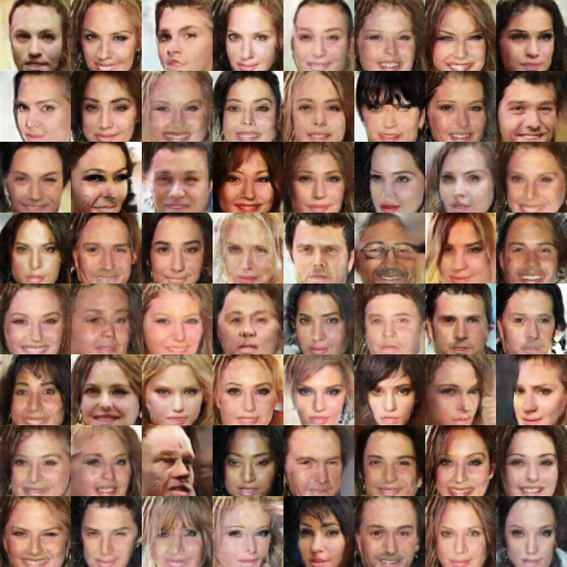
Your final deliverable is two images. The first should be a set of randomly generated faces. This is as simple as generating random z variables, and then running them through your generator.

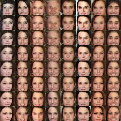
For the second image, you must pick two random z values, then linearly interpolate between them (using about 8-10 steps). Plot the face corresponding to each interpolated z value.

See the beginning of this lab spec for examples of both images.

The reference implementation was trained for 8 hours on a GTX 1070. It ran for 25 epochs (ie, scan through all 200,000 images), with batches of size 64 (3125 batches / epoch).

Although, it might work with far fewer (ie, 2) epochs…