BYU CS classes

To understand expectation maximization, and to explore how to learn the parameters of a Gaussian mixture model.

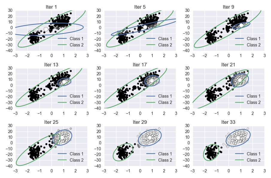
For this lab, you will implement the Expectation Maximization algorithm on the Old Faithful dataset. This involves learning the parameters of a Gaussian mixture model. Your notebook should produce a visualization of the progress of the algorithm. The final figure should look something like this:

Your notebook will be

In order to visualize a covariance matrix, you should plot an ellipse representing the 95% confidence bounds of the corresponding Gaussian. Here is some code that accepts as input a covariance matrix, and returns a set of points that define the correct ellipse; these points can be passed directly to the plt.plot() command as the x and y parameters.

import numpy as np
 
def cov_to_pts( cov ):
    circ = np.linspace( 0, 2*np.pi, 100 )
    sf = np.asarray( [ np.cos( circ ), np.sin( circ ) ] )
    [u,s,v] = np.linalg.svd( cov )
    pmat = u*2.447*np.sqrt(s) # 95% confidence
    return np.dot(  pmat, sf )