BYU CS classes

To understand expectation maximization, and to explore how to learn the parameters of a Gaussian mixture model.

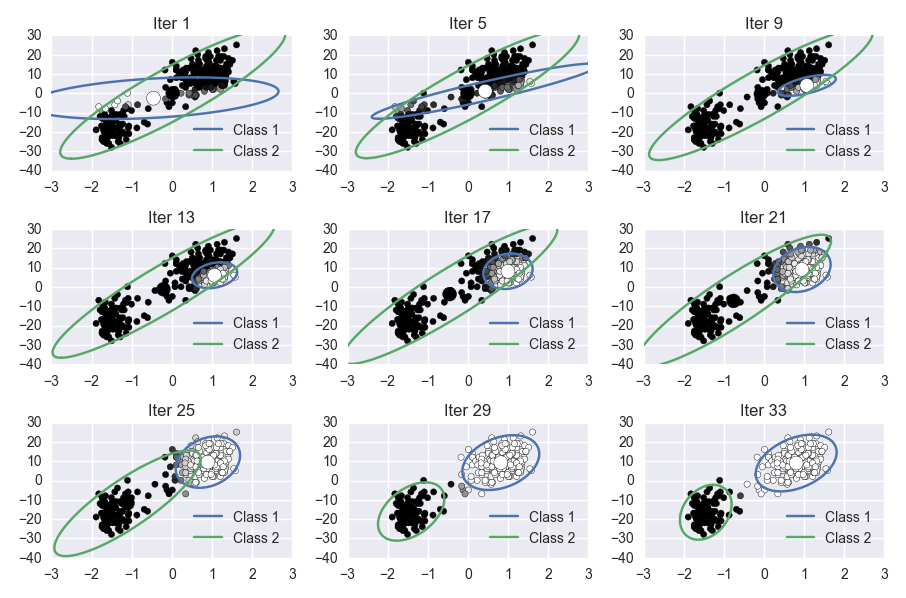
For this lab, you will implement the Expectation Maximization algorithm on the Old Faithful dataset. This involves learning the parameters of a Gaussian mixture model. Your notebook should produce a visualization of the progress of the algorithm. The final figure should look something like this:

Your notebook will be graded on the following elements:

• 10% Data is correctly mean-centered
• 20% Correctly updates responsibilities
• 20% Correctly updates means
• 20% Correctly updates covariances
• 20% Correctly updates mixing weights
• 10% Final plot is tidy and legible

For this lab, you will use the Old Faithful dataset, which you can download here:

Old Faithful dataset

To help our TA better grade your notebook, you should use the following initial parameters:

# the Gaussian means (as column vectors -- ie, the mean for Gaussian 0 is mus[:,0]
mus = np.asarray( [[-1.17288986, -0.11642103],
                   [-0.16526981,  0.70142713]])
 
# the Gaussian covariance matrices
covs = list()
covs.append( 
    np.asarray([[ 0.74072815,  0.09252716],
                [ 0.09252716,  0.5966275 ]]) )
covs.append( 
    np.asarray([[ 0.39312776, -0.46488887],
                [-0.46488887,  1.64990767]]) )
 
# The Gaussian mixing weights
mws = [ 0.68618439, 0.31381561 ]

In order to visualize a covariance matrix, you should plot an ellipse representing the 95% confidence bounds of the corresponding Gaussian. Here is some code that accepts as input a covariance matrix, and returns a set of points that define the correct ellipse; these points can be passed directly to the plt.plot() command as the x and y parameters.

import numpy as np
 
def cov_to_pts( cov ):
    circ = np.linspace( 0, 2*np.pi, 100 )
    sf = np.asarray( [ np.cos( circ ), np.sin( circ ) ] )
    [u,s,v] = np.linalg.svd( cov )
    pmat = u*2.447*np.sqrt(s) # 95% confidence
    return np.dot(  pmat, sf )

Here are some additional python functions that may be helpful to you:

# compute the likelihood of a multivariate Gaussian
scipy.stats.multivariate_normal.pdf
 
# scatters a set of points; check out the "c" keyword argument to change color, and the "s" arg to change the size
plt.scatter
plt.xlim # sets the range of values for the x axis
plt.ylim # sets the range of values for the y axis
 
# to check the shape of a vector, use the .shape member
foo = np.random.randn( 100, 200 )
foo.shape # an array with values (100,200)
 
# to transpose a vector, you can use the .T operator
foo = np.atleast_2d( [42, 43] ) # this is a row vector
foo.T # this is a column vector
 
import numpy as np
np.atleast_2d
np.sum