This is an old revision of the document!
Table of Contents
Objective:
To understand the relationship between a prior, a likelihood, a posterior and the posterior predictive distribution. To understand that distributions can be placed over arbitrary objects, including things like abstract sequences of numbers.
Deliverable:
For this lab, you will turn in an ipython notebook that implements the “Bayesian Concept Learning” model from Chapter 3 of MLAPP.
Your notebook should perform the following functions:
- Prompt the user for a set of numbers. (What happens if they only enter one number?)
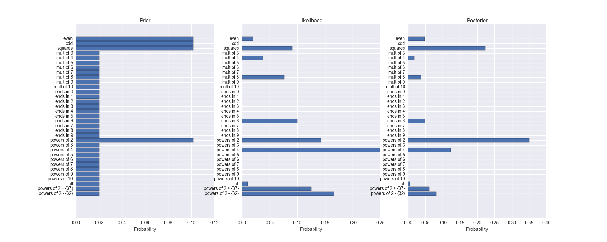
- Display the prior, likelihood, and posterior for each concept
- Print the most likely concept
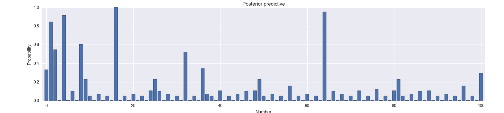
- Print the posterior predictive distribution over numbers
When you display your prior, likelihood, and posterior, your figure should look something like the ones in the book; my version is shown here:
Similarly, when you display the posterior predictive, your figure should look something like this:
Description:
Following the Bayesian Concept Learning example in Chapter 3 of MLAPP, we're interested in reasoning about the origin of a set of numbers. We'll do this by placing a prior over a set of possible concepts (or “candidate origins”), and then use Bayes' law to construct a posterior distribution over concepts given some data.
For this lab, we will only consider numbers between 0 and 100.
Your notebook should construct a set of possible number-game concepts (such as “even” or “odd”). These can be any set of concepts you want, but should include at least all of the concepts in the book (see, for example, Fig. 3.2). You must assign a prior probability to each concept; the prior can be anything you want. This is
$$p(h)$$
You must then prompt the user for some data. This will just be a sequence of numbers, like 16, 2,4,6 or 4,9,25. This is $\mathrm{data}$. You must then compute the likelihood of the $\mathrm{data}$, given the hypothesis:
$$p(\mathrm{data} | h )$$
Important: you can assume that each number in the data was sampled independently, and that each number was sampled uniformly from the set of all possible numbers in that concept.
Hint: what does that imply about the probability of sampling a given number from a concept with lots of possibilities, such as the all concept, vs. a concept with few possibilities, such as multiples of 10?
Prepare a figure, as described in the Deliverable that illustrates your prior, the likelihood of the data for each concept, the posterior. Note: distributions should be properly normalized.
You must also prepare a figure showing the posterior predictive distribution. This distribution describes the probability that a number $\tilde{x}$ is in the target hypothesis, given the data. The book is somewhat unclear on this, but to do this, we marginalize out the specific hypothesis:
$$p(\tilde{x} \in C | \mathrm{data} ) = \sum_h p(\tilde{x} \in C , h | \mathrm{data} )$$
$$p(\tilde{x} \in C | \mathrm{data} ) = \sum_h p(\tilde{x} \in C | h) p( h | \mathrm{data} )$$
We've already computed the posterior $p( h | \mathrm{data} )$, so we're only left with the term $p(\tilde{x} \in C | h)$. For this, just use an indicator function that returns 1 if $\tilde{x}$ is in $h$, and 0 otherwise.
Hint: just like any other distribution, the posterior predictive is normalized - but it is not normalized as a function of $\tilde{x}$. So what is it normalized over?
Hints:
When using an ipython notebook, it's nice to make your plots show up inline. To do this, add the following lines to the first cell of your notebook:
# this tells seaborn and matplotlib to generate plots inline in the notebook
%matplotlib inline

# these two lines allow you to control the figure size
%pylab inline
pylab.rcParams['figure.figsize'] = (16.0, 8.0)
You may find the following functions useful:
input('Please enter a set of numbers: ')

len

range

filter

map

all

import matplotlib.pyplot as plt
import seaborn
plt.figure( 42 )
plt.clf()
plt.subplot

plt.barh
plt.title
plt.xlabel
