BYU CS classes

To understand how to sample from different distributions, and to understand the link between samples and a PDF/PMF. To explore different parameter settings of common distributions, and to implement a small library of random variable types.

You should turn in an ipython notebook that implements and tests a library of random variable types.

When run, this notebook should sample multiple times from each type of random variable; these samples should be aggregated and visualized, and compared to the corresponding PDF/PMF. The result should look something like this:

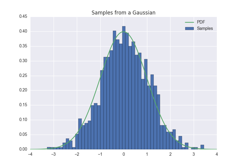
For multidimensional variables, your visualization should convey information in a natural way; you can either use 3d surfaces, or 2d contour plots:

You must implement a random variable object. These should all inherit from a base random variable object:

class RandomVariable:
    def __init__( self ):
        self.state = None
        pass
 
    def get( self ):
        return self.state
 
    def sample( self ):
        pass
 
    def ll( self ):
        return NaN
 
    def propose( self ):
        pass
 

For example, your univariate Gaussian class might look like this:

class Gaussian( RandomVariable ):
    def __init__( self, mu, sigma ):
        self.mu = mu
        self.sigma = sigma
        self.state = 0
 
    def sample( self ):
        return self.mu + self.sigma * numpy.Random.randn()
 
    def ll( self ):
        return 
 

* The following one dimensional, continuous valued distributions. For these, you should also plot the PDF of the random variable on the same plot; the curves should match. Note: it is not sufficient to let seaborn estimate the PDF using its built-in KDE estimator; you need to plot the true PDF. In other words, you can't just use seaborn.kdeplot!

• Beta (alpha=1, beta=3)
• Poisson (lambda=7)
• Univariate Gaussian (mean=2, variance=3)

* The following discrete distributions. For these, plot predicted and empirical histograms side-by-side:

• Bernoulli (p=0.7)
• Multinomial (theta=[0.1, 0.2, 0.7])

* The following multidimensional distributions. For these,

• Two-dimensional Gaussian
• 3-dimensional Dirichlet

The following functions may be useful to you:

matplotlib.pyplot.contour
 
seaborn.kdeplot
 
seaborn.jointplot
 
hist( data, bins=50, normed=True )
 
numpy.linspace
 
legend
 
title