Table of Contents
Objective:
To code a simple gradient descent based optimizer, to solidify understanding of score and loss functions, to improve ability to vectorize code, and to learn about numerical differentiation.
Deliverable:
You should turn in an iPython notebook that implements vanilla gradient descent on a 10-way CIFAR classifier. You should load the CIFAR-10 dataset, create a linear score function, and use the log soft-max loss function.
To optimize the parameters, you should use vanilla gradient descent.
To calculate the gradients, you should use numerical differentiation. Because we didn't cover this in class, you will need to read up on it; resources are listed below.
Your code should be fully vectorized. There should only be two Clarification: You will have code for both calculating a score function, and a loss function. You are not allowed to use for loops in your code: one that iterates over steps in the gradient descent algorithm, and one that loops over parameters to compute numerical gradients.for loops in either one! However, there may be other places in your code where for loops are unavoidable - for example, the outermost loop (that is running the gradient descent algorithm) needs a for loop, and you may also need to use a for loop to iterate over the parameters as you calculate the gradients (I actually used two for loops - one to iterate over rows of the W matrix, and one to iterate over columns).
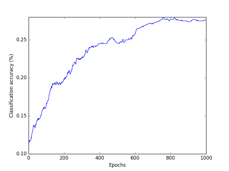
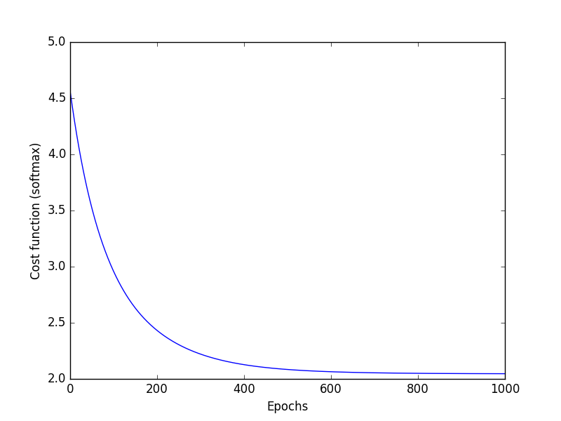
Your notebook should display two plots: classification accuracy over time, and the loss function over time. Please cleanly label your axes!
Example plots are shown at the right.
The CIFAR-10 dataset can be downloaded at https://www.cs.toronto.edu/~kriz/cifar.html
Note: make sure to download the python version of the data - it will simplify your life!
Grading standards:
Your notebook will be graded on the following:
- 20% Correct implementation of score function
- 20% Correct implementation of loss function
- 20% Correct implementation of gradient descent
- 20% Fully vectorized code
- 10% Tidy and legible visualization of cost function
- 10% Tidy and legible plot of classification accuracy over time
- +5% Complete auto gradient decent lab
Description:
We have discussed linear score functions and two different loss functions - but we have not said how we should adjust the parameters W to improve our classification accuracy (or minimize our loss). We will now optimize W by computing the gradient of the loss function with respect to our parameters, and then follow the slope downhill to achieve a better and better loss.
Where do gradients come from? We will have much to say about that later in the class, but for now we will rely on an (inefficient!) technique called numerical differentiation. We didn't cover this in class, but the concept is simple, so you'll need to do a little bit of out-of-class reading to learn the technique.
Because numerical differentiation is computationally intensive, we will simplify our dataset a little bit, as shown below.
With the gradient in hand, you should implement the vanilla gradient descent algorithm, as described in class and repeated here:
step_size = 0.1
for i in range(0,NUM_EPOCHS):
    loss_function_value, grad = numerical_gradient( loss_function, W )
    W = W - step_size * grad
Note a couple of things about this code: first, it is fully vectorized. Second, the numerical_gradient function accepts a parameter called loss_function – numerical_gradient is a higher-order function that accepts another function as an input. This numerical gradient calculator could be used to calculate gradients for any function. Third, you may wonder why my loss_function doesn't need the data! Since the data never changes, I curried it into my loss function, resulting in a function that only takes one parameter – the matrix W.
You should run your code for 1000 epochs. (Here, by epoch, I mean “step in the gradient descent algorithm.”). Note, however, that for each step, you have to calculate the gradient, and in order to calculate the gradient, you will need to evaluate the loss function many times.
You should plot both the loss function and the classification accuracy at each step.
Preparing the data:
Because numerical differentiation is so computationally intensive, we will simplify the dataset a lot. First, we will only use the first 1000 images; second, we will randomly project those images into a small 10 dimensional space (!). Our linear parameter W will therefore be 10×10, for a total of 100 parameters. We will also whiten the data, to help improve convergence and numerical stability.
# =============================================
#
# load cifar-10-small and project down
#

def unpickle( file ):
    import cPickle
    fo = open(file, 'rb')
    dict = cPickle.load(fo)
    fo.close()
    return dict

data = unpickle( 'cifar-10-batches-py/data_batch_1' )

features = data['data']
labels = data['labels']
labels = np.atleast_2d( labels ).T

N = 1000
D = 10

# only keep N items
features = features[ 0:N, : ]
labels = labels[ 0:N, : ]

# project down into a D-dimensional space
features = np.dot( features, np.random.randn( 3072, D) )

# whiten our data - zero mean and unit standard deviation
features = (features - np.mean(features, axis=0)) / np.std(features, axis=0)
Calculating scores and losses
You should use a linear score function, as discussed in class. This should only be one line of code!
You should use the log softmax loss function, as discussed in class. For each training instance, you should compute the probability that the instance i is classified as class k, using p(instance i = class k) = exp( s_ik ) / sum_j exp( s_ij ) (where s_ij is the score of the i'th instance on the j'th class), and then calculate L_i as the log of the probability of the correct class. Your overall loss is then the mean of the individual L_i terms.
Note: you should be careful about numerical underflow! To help combat that, you should use the log-sum-exp trick (or the exp-normalize trick):
Calculating numerical gradients
Remember the definition of a gradient: it is a vector (or matrix) of partial derivatives. We can think of the loss function as a function that maps W to a single scalar – the loss. Intuitively, you can think of the gradient as the answer to the following question: for each parameter, what would happen to the loss if I held everything else constant, and twiddled just this one parameter a little bit?
Numerical differentiation is the literal instantiation of this idea: for each parameter, we calculate the loss, then we twiddle each parameter just a little bit (by delta), and the recalculate the loss.
Hint: how many times must we compute the loss in order to calculate a gradient for a function with 100 parameters?
I used a delta of 0.000001.
Please feel free to search around online for resources to understand this better. For example:
These lecture notes (see eq. 5.1)
Wikipedia's entry on numerical differentiation isn't too bad, although only the first bit is helpful for this lab.
Hints:
You should test your numerical gradient calculator on known test cases - for example, f(x)=x^2.
Here are some functions that may be helpful to you:
np.argmax
np.sum
np.exp
np.log
np.mean
np.random.randn
Note that many of these functions accept two useful arguments: axis=, which specifies which axis you want to operate on, and keepdims=True, which ensures that the result has broadcastable dimensions.
You may find this tutorial on pyplot helpful.
Extra credit:
You may complete the old lab 04 for 5% of extra credits. http://liftothers.org/dokuwiki/doku.php?id=cs501r_f2016:lab4
