Table of Contents
BYU CS 501R - Deep Learning:Theory and Practice - Lab 6
Objective:
To build a dense prediction model, to begin to read current papers in DNN research, to experiment with different DNN topologies, and to experiment with different regularization techniques.
Deliverable:

For this lab, you will turn in a report that describes your efforts at creating a tensorflow radiologist. Your final deliverable is either a notebook or PDF writeup that describes your (1) topology, (2) cost function, (3) method of calculating accuracy, and (4) results with experimenting with regularization. You should also report on how much of the data you used.
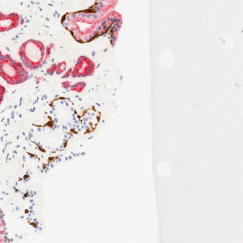
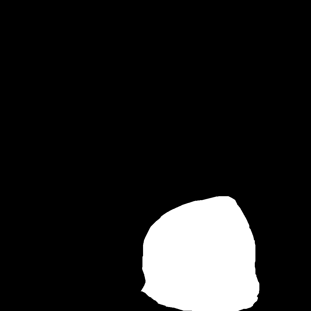
Your notebook / writeup should also include at an image that
shows the dense prediction produced by your network on the
pos_test_000072.png image. This is an image in the test set that
your network will not have seen before. This image, and the ground truth labeling, is shown at the right. (And is contained in the downloadable dataset below).
Grading standards:
Your notebook will be graded on the following:
- 30% Proper design, creation and debugging of a dense prediction network
- 30% Proper design of a loss function and test set accuracy measure
- 20% Proper experimentation with two different regularizers
- 20% Tidy visualization of the output of your dense predictor
Data set:

The data is given as a set of 1024×1024 PNG images. Each input image
(in the inputs directory) is an RGB image of a section of tissue,
and there a file with the same name (in the outputs directory) that
has a dense labeling of whether or not a section of tissue is
cancerous (white pixels mean “cancerous”, while black pixels mean “not
cancerous”).
The data has been pre-split for you into test and training splits.
Filenames also reflect whether or not the image has any cancer at all
(files starting with pos_ have some cancerous pixels, while files
starting with neg_ have no cancer anywhere). All of the data is
hand-labeled, so the dataset is not very large. That means that
overfitting is a real possibility.
The data can be downloaded here. Please note that this dataset is not publicly available, and should not be redistributed.
As in the previous lab, you are welcome to sub-sample the data if your computer is not powerful enough to fit it all in RAM. However, if you do, please clearly report how much data you used in your final report.
Description:
For this lab, you will implement a virtual radiologist. You are given images of possibly cancerous tissue samples, and you must build a detector that identifies where in the tissue cancer may reside.
For this lab, there are two primary tasks:
Part 1: Implement a dense predictor
In previous labs and lectures, we have talked about DNNs that classify an entire image as a single class. Here, however, we are interested in a more nuanced classification: given an input image, we would like to identify each pixel that is possibly cancerous. That means that instead of a single output, your network should output an “image”, where each output pixel of your network represents the probability that a pixel is cancerous.
Part 1a: Implement your network topology
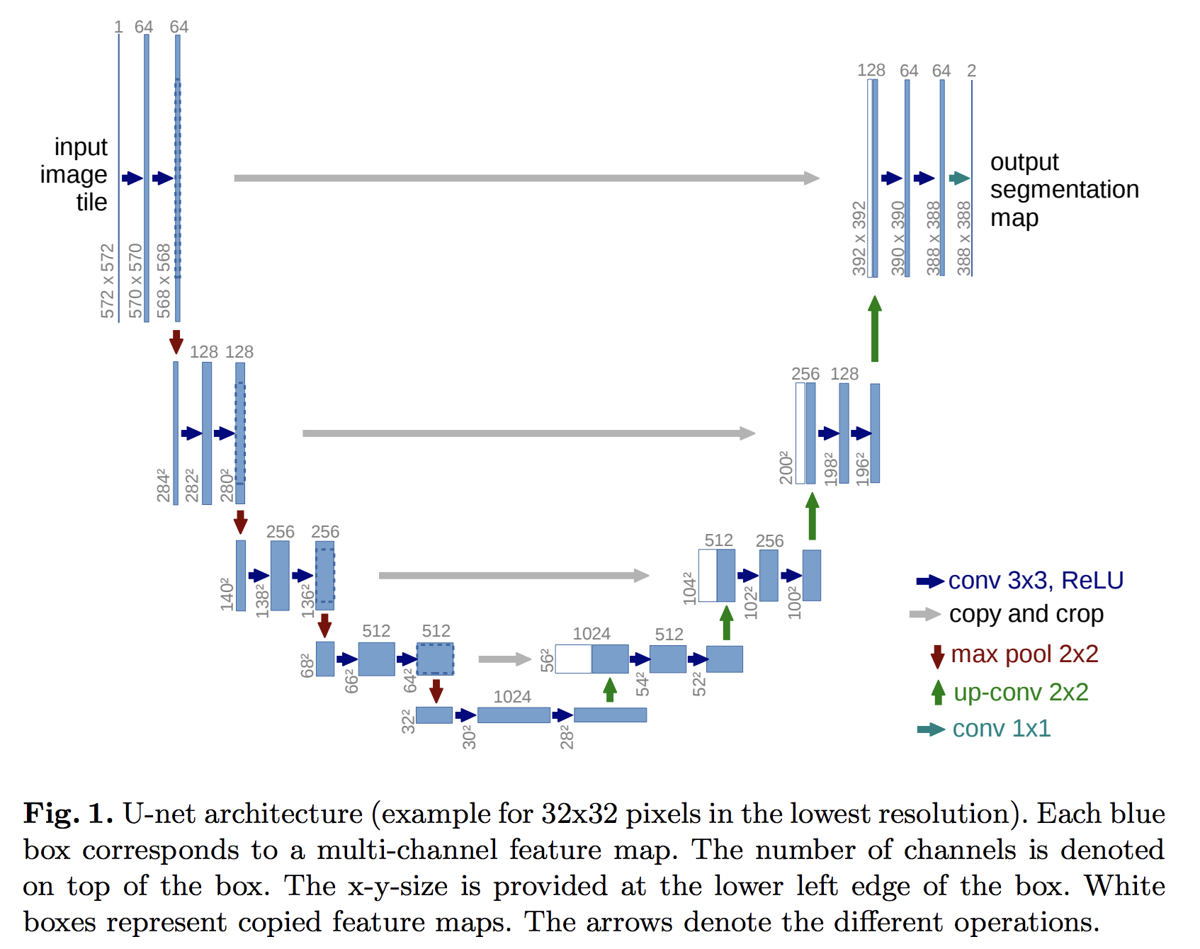
Like the previous lab, you must choose your topology. I have had good
luck implementing the “Deep Convolution U-Net” from this paper: U-Net: Convolutional Networks for Biomedical Image Segmentation (See figure 1, replicated at the right). This should be fairly easy to implement given the
conv helper functions that you implemented previously; you
may also need the tensorflow function tf.concat.
Note that the simplest network you could implement (with all the desired properties) is just a single convolution layer with two filters and no relu! Why is that? (of course it wouldn't work very well!)
Part 1b: Implement a cost function
You should still use cross-entropy as your cost function, but you may need to think hard about how exactly to set this up – your network should output cancer/not-cancer probabilities for each pixel, which can be viewed as a two-class classification problem.
Part 2: Test two regularizers
To help combat overfitting, you should implement some sort of regularization. This can be either dropout, or L1 / L2 regularization.
First, you must construct a baseline performance measure without regularization. This is straightforward: you must simply test classification accuracy on the held-out test set, and compare it to the accuracy of the training set. The difference is the “generalization error.”
You must experiment with two different regularizers. For each, train your network, and then report on the following questions:
- What is the final classification accuracy on the test set before and after regularization?
- Is the generalization error better or worse?
- If you used dropout, what dropout probability did you use?
- If you used L1/L2, how did you pick lambda?
Hints:
You are welcome to resize your input images, although don't make them so small that the essential details are blurred! I resized my images down to 512×512.
I used the scikit-image package to handle all of my image IO and
resizing. NOTE: be careful about data types! When you first load
an image using skimage.io.imread, it returns a tensor with uint8
pixels in the range of [0,255]. However, after using
skimage.transform.resize, the result is an image with float32
entries in [0,1].
Don't forget to whiten your data. And remember that if your data is stored as a numpy array, be careful about the data type: if you try to whiten it while it is still a uint8, bad things will happen.
You are welcome (and encouraged) to use the built-in tensorflow dropout layer.
