BYU CS classes

• To build a dense prediction model
• To begin reading current papers in DNN research

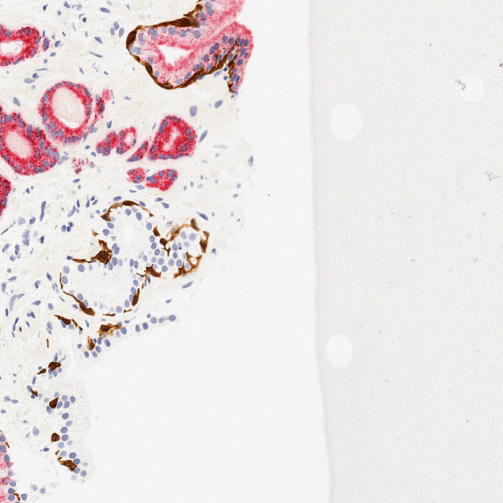
For this lab, you will turn in a notebook that describes your efforts at creating a pytorch radiologist. Your final deliverable is a notebook that has (1) deep network, (2) cost function, (3) method of calculating accuracy, (4) an image that shows the dense prediction produced by your network on the pos_test_000072.png image. This is an image in the test set that your network will not have seen before. This image, and the ground truth labeling, is shown at the right. (And is contained in the downloadable dataset below).

Your notebook will be graded on the following:

• 40% Proper design, creation and debugging of a dense prediction network
• 40% Proper design of a loss function and test set accuracy measure
• 10% Tidy visualizations of loss of your dense predictor during training
• 10% Test image output

The data is given as a set of 1024×1024 PNG images. Each input image (in the inputs directory) is an RGB image of a section of tissue, and there a file with the same name (in the outputs directory) that has a dense labeling of whether or not a section of tissue is cancerous (white pixels mean “cancerous”, while black pixels mean “not cancerous”).

The data has been pre-split for you into test and training splits. Filenames also reflect whether or not the image has any cancer at all (files starting with pos_ have some cancerous pixels, while files starting with neg_ have no cancer anywhere). All of the data is hand-labeled, so the dataset is not very large. That means that overfitting is a real possibility.

The data can be downloaded here. Please note that this dataset is not publicly available, and should not be redistributed.

For this lab, you will implement a virtual radiologist. You are given images of possibly cancerous tissue samples, and you must build a detector that identifies where in the tissue cancer may reside.

Part 1: Implement a dense predictor

In previous labs and lectures, we have talked about DNNs that classify an entire image as a single class. Here, however, we are interested in a more nuanced classification: given an input image, we would like to identify each pixel that is possibly cancerous. That means that instead of a single output, your network should output an “image”, where each output pixel of your network represents the probability that a pixel is cancerous.

Part 1a: Implement your network topology

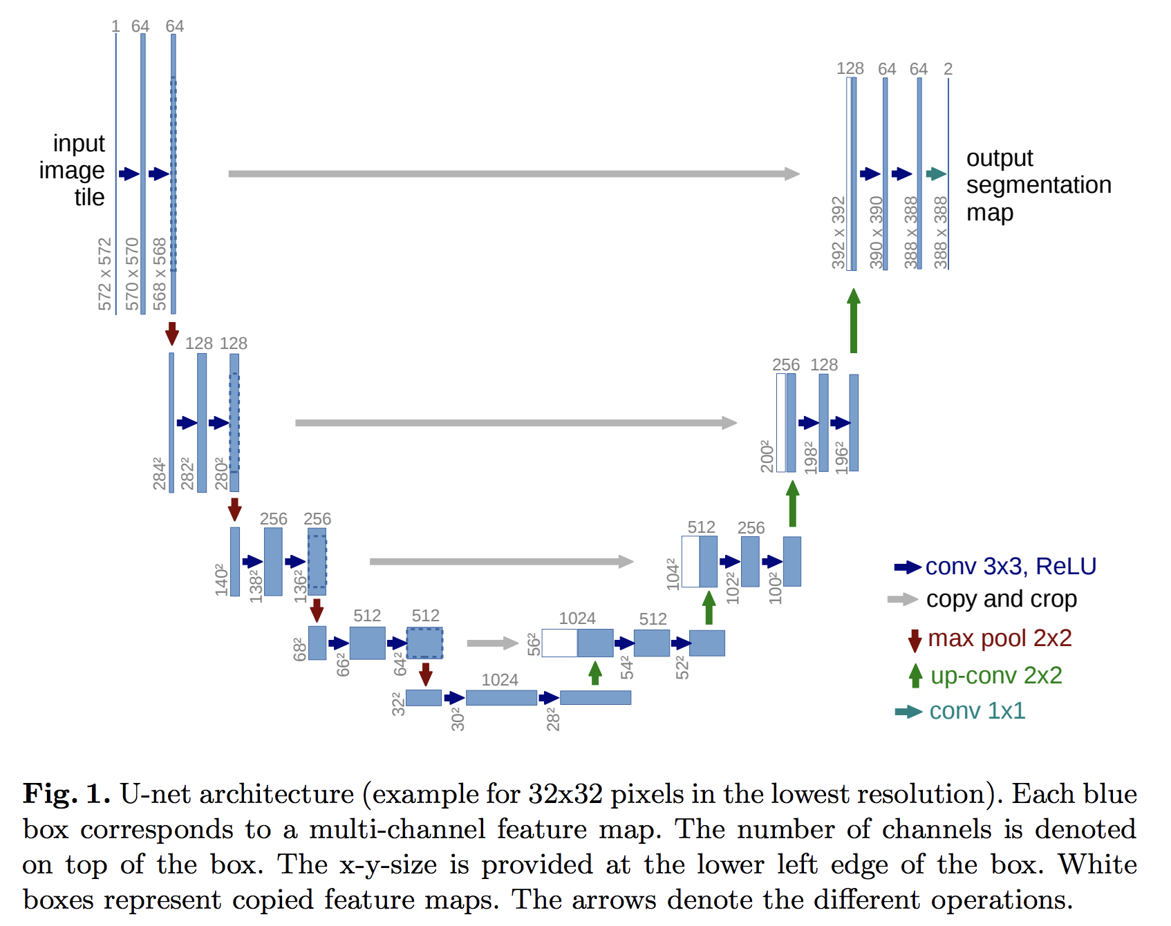
Use the “Deep Convolution U-Net” from this paper: U-Net: Convolutional Networks for Biomedical Image Segmentation (See figure 1, replicated at the right). This should be fairly easy to implement given the conv helper functions that you implemented previously; you may also need the pytorch function torch.cat and nn.ConvTranspose2d

torch.cat allows you to concatenate tensors. nn.ConvTranspose2d is the opposite of nn.Conv2d. It is used to bring an image from low res to higher res. This blog should help you understand this function in detail.

Note that the simplest network you could implement (with all the desired properties) is just a single convolution layer with two filters and no relu! Why is that? (of course it wouldn't work very well!)

Part 1b: Implement a cost function

You should still use cross-entropy as your cost function, but you may need to think hard about how exactly to set this up – your network should output cancer/not-cancer probabilities for each pixel, which can be viewed as a two-class classification problem.

Part 2: Plot performance over time

Please generate a plot that shows loss on the training set as a function of training time. Make sure your axes are labeled!

Part 3: Generate a prediction on the pos_test_000072.png image

Calculate the output of your trained network on the pos_test_000072.png image, then make a hard decision (cancerous/not-cancerous) for each pixel. The resulting image should be black-and-white, where white pixels represent things you think are probably cancerous.

Importing data is a little tricky for this lab. There are a few ways to handle data. I downloaded the dataset and divided it into train_input, train_output, test_input and test_output. I uploaded this to my google drive and wrote the follwoing in colab to use the dataset

    # Load the Drive helper and mount
    from google.colab import drive
    # This will prompt for authorization.
    drive.mount('/content/drive')
    print('done')

This will ask you for an authentication so please copy paste the code that it gives you. Next make your dataset class and you will be using ''ImageFolder' to build your dataset in init:

    class CancerDataset(Dataset):
      def __init__(self, dataset_folder):
        self.dataset_folder = torchvision.datasets.ImageFolder(dataset_folder + 'train_input' ,transform = transforms.ToTensor())
        self.label_folder = torchvision.datasets.ImageFolder(dataset_folder + 'train_output' ,transform = transforms.ToTensor())
 
      def __getitem__(self,index):
        img = self.dataset_folder[index]
        label = self.label_folder[index]
        return img[0],label[0]
 
      def __len__(self):
        return len(self.dataset_folder)

Finally you can call your dataset like this:

    trainset = CancerDataset(dataset_folder = '/content/drive/My Drive/cancer_data/')

The tricky part here is that Imagefolder takes a folder of images. When you have both inputs and outputs folder inside cancer_data, it does not know that outputs is label. To get over this problem, I created a layer of folders that looks like this: cancer_data → train_input → train_input→all image files and similar for all other folders.(we are looking at other options of making the dataset…)

You are welcome to resize your input images, although don't make them so small that the essential details are blurred! I resized my images down to 512×512.

You are welcome (and encouraged) to use the built-in dropout layer.